Predicting cancer risk using machine learning on lifestyle and genetic data

Dataset presentation

The dataset used in this study consists of 1,200 patient records were collected in an Excel file having structured labelled columns for different clinical and lifestyle data, this study used a subset of the publicly available Cancer Prediction Dataset (1,200 out of 1,500 samples), which is shared under the Attribution 4.0 International (CC BY 4.0) license³². Every row is an individual patient and every column relays a certain feature for risk and diagnosis of cancer. The dataset includes a total of nine features, in addition to the target variable used for prediction. A detailed description of all features and their types is provided in Table 2.

The diagnosis variable is the target of prediction in this study. It facilitates the categorization of patients according to their cancer diagnosis status. The dataset is equitably distributed among the characteristics and the target class, hence facilitating an impartial training procedure for ML models.

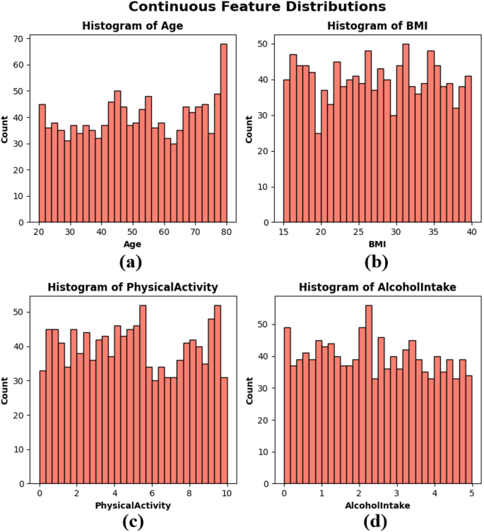
Frequency distributions charts which are called Histograms were created of Age, BMI, Physical activity and Alcohol intake to visualize the distribution of continuous variables in the dataset. These factors represent important aspects of an individual’s health and life that could be related to cancer risk. The age distribution in subplot Fig. 2(a) is predominantly uniform across the 20 to 80 range, with a modest increase in frequency among older people. The BMI distribution in subplot Fig. 2(b) is uniformly distributed between 15 and 40, signifying a heterogeneous patient population regarding body composition. Physical activity in subplot Fig. 2(c) exhibits variability throughout the population, with significant frequencies observed across all levels from 0 to 10 h per week. The alcohol consumption depicted in subplot Fig. 2(d) has a uniform distribution ranging from 0 to 5 units, devoid of significant grouping. The histograms illustrate that the dataset exhibits authentic variability and is well-balanced, essential for constructing robust and generalizable ML models, as seen in Fig. 2.

Histograms of continuous features — (a) Age, (b) BMI, (c) Physical activity, and (d) Alcohol intake.

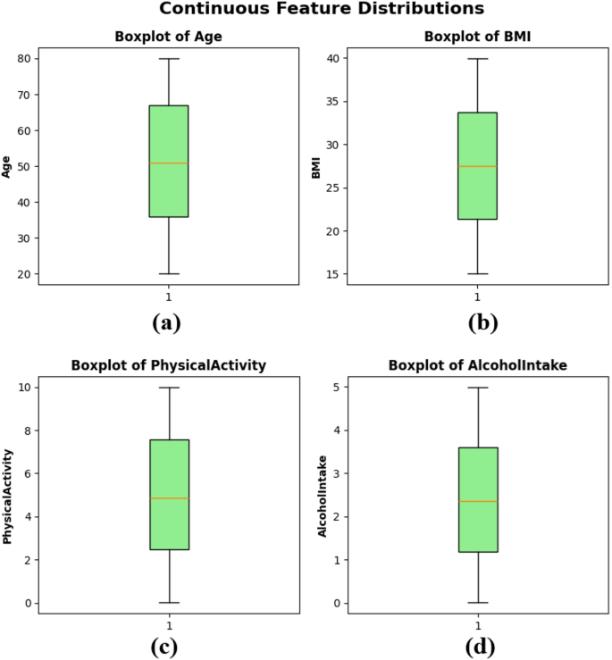
Boxplots were created to illustrate the distribution, central tendency, and possible outliers of the continuous variables in the dataset. Figure 3(a) depicts an age distribution with a median of roughly 50 years, an Interquartile Range (IQR) of about 35 to 65, and the absence of extreme outliers. The BMI feature in subplot Fig. 3(b) shows a balanced distribution, with the middle value around 27 and a narrow IQR, indicating similar body composition values among the sample. Physical activity in subplot Fig. 3(c) ranges from 0 to 10 h per week, with a median close to 5, reflecting a balanced distribution of physical activity levels among patients. Lastly, alcohol intake in subplot Fig. 3(d) also shows a wide distribution from 0 to 5 units per week, with a median slightly above 2 units. The boxplots indicate that the dataset is free of significant skewness or extreme outliers in the continuous features, supporting its suitability for training models in ML, as presented in Fig. 3.

Boxplots of continuous features — (a) Age, (b) BMI, (c) Physical Activity, and (d) Alcohol Intake.

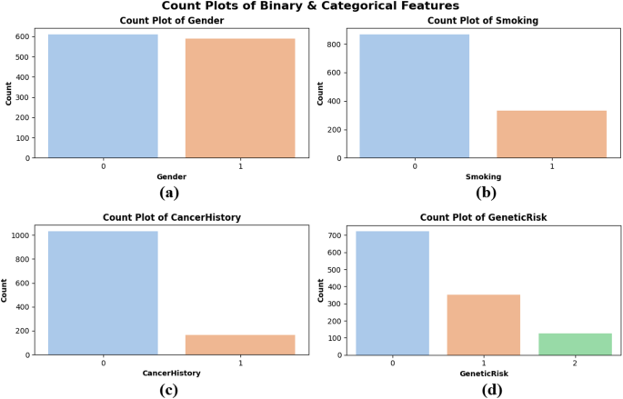
Count plots were created to assess the distribution of categorical and binary data, specifically for Gender, Smoking, CancerHistory, and GeneticRisk. Figure 4 illustrates that the gender distribution in subplot Fig. 4(a) is nearly balanced between males (0) and females (1), signifying equitable representation across sexes. Figure 4(b) illustrates that a greater proportion of patients are non-smokers, potentially indicating lifestyle trends among the population. In sidebar Fig. 4(c), most patients indicate no personal history of cancer, whereas a smaller nevertheless notable proportion has been previously diagnosed. The genetic risk factor in subplot Fig. 4(d) is classified into low (0), medium (1), and high (2) levels. The majority of patients are categorized as low-risk, although a smaller number are deemed high-risk. These plots illustrate the dataset’s balanced characteristics and authentic variability, confirming that the model is trained on a representative sample, as depicted in Fig. 4.

Count plots of binary and categorical features — (a) Gender, (b) Smoking, (c) Cancer History, and (d) Genetic Risk.

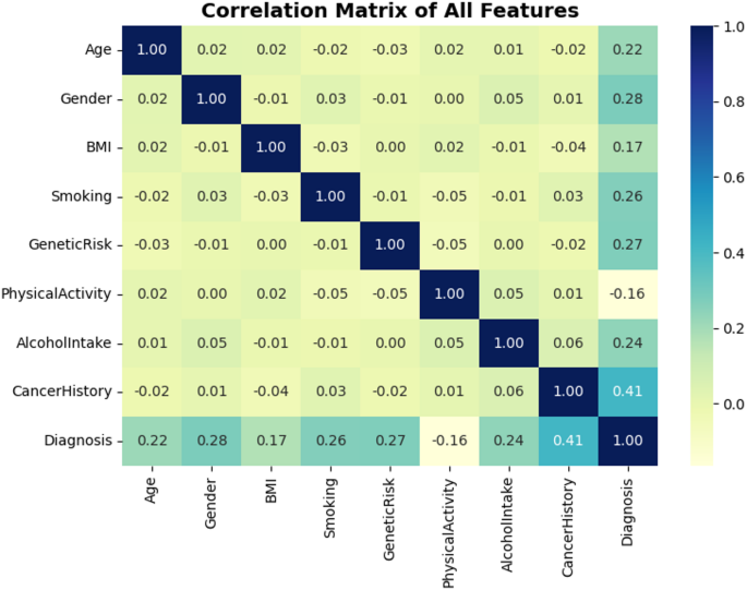
The matrix correlation gives statistical readings over each linear relationship between either features in the dataset and the target (Diagnosis). As can be seen from Fig. 5, CancerHistory has the highest correlation with the target and the correlation value is 0.41. This implies a mild linear relationship, or in other words, the patients who had cancer in past are more likely to have cancer in the future, as it is clinically more relevant. Other features exhibiting a high correlation with the target variable include Gender (0.28), GeneticRisk (0.27) and Smoking (0.26). While most of the feature pairs exhibit weak or negligible correlations—such as BMI and GeneticRisk or Age and PhysicalActivity—This diversity demonstrates the multi-dimensionality of the dataset, and justifies utilizing non-linear models to capture complex interactions. The above correlation observations in Fig. 5 affirm the importance of the chosen features as they are justified to have further impact in the predictive modeling.

Correlation matrix of all features including diagnosis.

Workflow overview

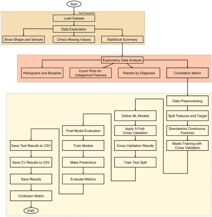
The methodology of this study follows a structured and data-driven approach to develop an accurate cancer prediction system using ML, as illustrated in Fig. 6. The process begins with loading the dataset, which contains various patient features such as age, gender, BMI, smoking status, genetic risk, physical activity, alcohol intake, and personal history of cancer, along with the target variable, diagnosis. After loading, the dataset undergoes thorough exploration to understand its structure and integrity. Basic information such as shape, sample rows, and missing values is examined, followed by statistical summaries that provide insight into the distribution of each feature. To deepen this understanding, EDA is conducted through visualizations including histograms, boxplots, and count plots, helping to identify patterns and anomalies. A correlation matrix is also generated to detect relationships among numeric variables.

Following exploration, data preprocessing is performed where the dataset is split into input features and the target label. Continuous features are standardized using StandardScaler to ensure uniform scaling across models. The core of the methodology lies in training multiple ML models—such as Logistic Regression (LR), Decision Tree (DT), RF, Gradient Boosting (GB), Support Vector Machines (SVMs), k-Nearest Neighbors (k-NN), CatBoost, eXtreme Gradient Boosting (XGBoost), and Light Gradient Boosting Machine (LightGBM)—using 5-fold stratified cross-validation. This ensures balanced and robust evaluation by assessing each model’s accuracy across different data splits. The model with the highest average cross-validation accuracy is selected as the best-performing model.

To further validate model performance, a train-test split is applied and all models are evaluated on unseen test data. Key metrics such as accuracy, precision, recall, and F1-score are calculated for each model, and confusion matrices are plotted to visualize their classification performance. All evaluation results are saved as CSV files to support reproducibility and reporting. Finally, a GUI is developed using Tkinter, allowing users to enter patient information and receive instant predictions from the trained model. This end-to-end workflow ensures that the system is not only accurate and reliable but also accessible and user-friendly for practical use.

End-to-end workflow of the cancer prediction system incorporating data exploration, model training, evaluation, and GUI deployment.

Evaluation metrics

In order to verify the efficacy of the developed ML models, some popular classification metrics were adopted. These measures help in having a full overview of the efficiency of each model in separating patients into those with and without the disease, a very important aspect in all the medical- related prediction tasks.

One of the indicators is in particular the accuracy which is defined as percentage of correctly classification predictions (both negative and positive) over all the predictions performed. This provides a general sense of model correctness, as presented in Eq. (1). However, accuracy alone may not be sufficient in medical datasets, particularly when the cost of FNs or FPs is high.

To gain deeper insight, precision and recall were also evaluated. Precision measures the proportion of True Positive (TP) cases among all positive predictions, which is crucial to minimize false alarms and avoid subjecting healthy individuals to unnecessary concern or follow-up procedures, as shown in Eq. (2). On the other hand, recall—also known as sensitivity—focuses on the ability of the model to correctly identify actual cancer cases, ensuring that as few positive cases as possible go undetected. This is calculated as described in Eq. (3). As there is usually a trade-off between precision and recall, this study used the F1-score to have a single performance score that balances both. This takes the harmonic mean of precision and recall, and is useful when there is a slight class imbalance or when FPs and FNs are both concerning. Mathematically, the F1-score is defined in Eq. (4).

Alongside these scalar metrics, a confusion matrix was created for each model to illustrate the quantities of TPs, True Negatives (TNs), FPs, and FNs. This facilitated a clear comprehension of the model’s performance across various prediction types.

Each model was initially assessed utilizing a 5-fold stratified cross-validation approach, which maintained the class distribution within each fold. This yielded a strong assessment of the model’s generalization ability. Subsequently, the models were assessed on a distinct 20% hold-out test set, and identical metrics were calculated to gauge their real-world predictive efficacy.